Three figures are shown below. The first figure shows a grid of points. You are free to choose a grid of any size and shape with any number of grid points. The second figure shows a self-avoiding path that visits all grid points. Here too, you can choose such a path yourself among many possibilites that exist. Once the path is chosen, you see which grid points interact, as shown by the array of dashed lines. Notice that all non-bonded grid points in the path interact. The third figure shows that some grid points are black. You need to choose which grid points should be black for the following problem.

In the problem you need to solve using continuous optimization, assume that you have (-2.3) kT units of energy if two black grid points interact; (-1) kT units of energy if a black and a white grid points interact; 0 energy if two white grid points interact. Your task is to assign black color to m grid points out of n where n is the total number of grid points and m (which is less than n) is the number of black grid points specified, in order to have lowest energy for the entire grid.
Clearly, this is a combinatorial problem. You can see how many combinations exist to assign black to m points out of n. If you enumerate all those combinations and compute energy, you can identify the one with the lowest energy. But you should not do that here as it is computationally expensive. So, let us make it a continuous problem, as follows.
Let us assign for the ith grid point a variable xi, which can take any value between 0 and 1. If it takes 0, it is a white point; if it takes 1 it is a black point. So, if you have n grid points, you have n such variables. Now, let us see how we can compute energy for intermediate values between 0 and 1.
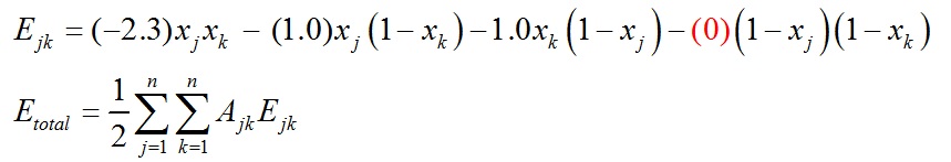
where Aij determines which grid points are interacting. If Ajk = 0, it means that j and k grid points are not interacting; if Ajk = 1, it means that j and k grid points are interacting.
Notice that the energy computation is correct when xi, i = 1 to n take 0 or 1. Notice also that the total energy is interpolated when the variables take values between 0 and 1.
Since Etotal is a continuous function, we can take derivatives and solve the sequence problem of assinging black and white colors to grid points using continous (i.e., gradient-based) optimization algorithms.
You may use Matlab's optimization tool-box for solving the problem.The following files will be useful to you to use "fmincon" routine in Matlab.
KKTdemo.m
obj.m
g1.m
What to submit:
You should submit on paper (not by email unless asked) the complete texttual description of what you have done, annotated figures and Matlab codes. Do not forget to include the optimization problem statement and all the data that you assumed.
Extra points for those who write a general program that handles any number of black points, any sized grid, 3D grid, etc.
